Literature review did not show any existing implementations of the EM algorithm for inverse Gaussian mixture models. Therefore, we must derive one from scratch.
As a model, the method given in Bilmes (1998, p. 3-7) is used. It shows the derivation of the EM equations for Normal mixture models.
The following variables are used:
\( \Theta \): the set of parameters estimates for the mixture model. \( \Theta^{g} \) refers to the ‘guessed’ parameter set.
\( \lambda_{\ell} \): the shape parameter for the \( \ell \)th mixture component
\( \mu_{\ell} \): the mean parameter for the \( \ell \)th mixture component
\( \alpha_{\ell} \): the mixture weight parameter for the \( \ell \)th mixture component
From Bilmes (1998, p. 2), we define:
$$ Q(\Theta,\Theta^{(i-1)})=E\left[\log p(X,Y|\Theta)|X,\Theta^{(i-1)}\right] $$
For the inverse Gaussian distribution, we have the following expression for the conditional probability of mixture component \( \ell \) given parameter guesses \( \lambda_{\ell} \) and \( \mu_{\ell} \) (Wikipedia, 2015a):
$$ p_{\ell}(x|\lambda_{\ell},\mu_{\ell})=\left[\frac{\lambda_{\ell}}{2\pi x^{3}}\right]^{1/2}\exp\frac{-\lambda_{\ell}(x-\mu_{\ell})^{2}}{2\mu^{2}x}\label{eq:probfunc}\tag{1} $$
We denote proportion of mixing components by \( \alpha_{\ell} \) in order to reduce confusion with the constant \( \pi \). We have the constraint that
$$ \sum_{\ell=1}^{M}\alpha_{\ell}=1 $$
The \( Q \) function is given by Bilmes (1998, p. 4):
$$ Q(\Theta,\Theta^{g})=\sum_{\ell=1}^{M}\sum_{i=1}^{N}\log(\alpha_{\ell})p(\ell|x_{i},\Theta^{g})+\sum_{\ell=1}^{M}\sum_{i=1}^{N}\log(p_{\ell}(x_{i}|\theta_{\ell}))p(\ell|x_{i},\Theta^{g})\label{eq:bilmes-eqn-5}\tag{2} $$
On each iteration, we need to improve the parameter estimates based on the previous estimates (Bilmes, 1998, p. 2):
$$ \Theta^{(i)}=argmax_{\Theta}Q(\Theta,\Theta^{(i-1)}) $$
The left-hand term of \( \eqref{eq:bilmes-eqn-5} \) is independent of the inverse Gaussian parameters and the right-hand term is independent of \( \alpha \). Therefore, we can reuse the result from Bilmes (1998, p. 5):
$$ \alpha_{\ell}^{new}=\frac{1}{N}\sum_{i=1}^{N}p(\ell|x_{i},\Theta^{g}) $$
We now need to maximise the following expression with respect to each of \( \lambda_{\ell} \) and \( \mu_{\ell} \)
$$ \sum_{\ell=1}^{M}\sum_{i=1}^{N}\log(p_{\ell}(x_{i}|\theta_{\ell}))p(\ell|x_{i},\Theta^{g})\label{eq:sumsum_logp}\tag{3} $$
Taking the log of \( \eqref{eq:probfunc} \), we get:
$$ \log p_{\ell}(x|\lambda_{\ell},\mu_{\ell}) = \log\left(\left[\frac{\lambda_{\ell}}{2\pi x^{3}}\right]^{1/2}\exp\frac{-\lambda_{\ell}(x-\mu_{\ell})^{2}}{2\mu^{2}x}\right) $$
$$ = \frac{1}{2}\log\left(\frac{\lambda_{\ell}}{2\pi x^{3}}\right)-\frac{\lambda_{\ell}(x-\mu_{\ell})^{2}}{2\mu^{2}x} $$
$$ = \frac{1}{2}\log(\lambda_{\ell})-\frac{1}{2}\log(2\pi x^{3})-\frac{\lambda_{\ell}(x-\mu_{\ell})^{2}}{2\mu^{2}x} $$
Substituting this into \( \eqref{eq:sumsum_logp} \), we get:
$$ \sum_{\ell=1}^{M}\sum_{i=1}^{N}(\frac{1}{2}\log(\lambda_{\ell})-\frac{1}{2}\log(2\pi x_{i}^{3})-\frac{\lambda_{\ell}(x_{i}-\mu_{\ell})^{2}}{2\mu^{2}x_{i}})p(\ell|x_{i},\Theta^{g})\label{eq:func-to-diff}\tag{4} $$
We wish to maximise \( \eqref{eq:func-to-diff} \) for \( \mu_{\ell} \), so we take its partial derivative with respect to \( \mu_{\ell} \) and set it equal to 0. Note that the first two terms inside the summations are independent of \( \mu_{\ell} \), so we can ignore them for the purpose of maximisation; we seek
$$ \frac{\partial}{\partial\mu_{\ell}}\sum_{i=1}^{N}\left[-\frac{\lambda_{\ell}(x_{i}-\mu_{\ell})^{2}}{2\mu^{2}x_{i}}\right]p(\ell|x_{i},\Theta^{g}) $$
$$ = -\lambda\frac{\partial}{\partial\mu_{\ell}}\sum_{i=1}^{N}\left[\frac{(x_{i}-\mu_{\ell})^{2}p(\ell|x_{i},\Theta^{g})}{2\mu^{2}x_{i}}\right]\label{eq:partial}\tag{5} $$
Concentrating just on the inner term of the summation, we need
$$ \frac{\partial}{\partial\mu_{\ell}}\frac{(x_{i}-\mu_{\ell})^{2}p(\ell|x_{i},\Theta^{g})}{2\mu^{2}x_{i}} $$
Apply the quotient rule:
$$ = \frac{2\mu_{\ell}^{2}x_{i}\left(-2x_{i}p(\ell|x_{i},\Theta^{g})+2\mu_{\ell}p(\ell|x_{i},\Theta^{g})\right)-4(x_{i}-\mu_{\ell})^{2}p(\ell|x_{i},\Theta^{g})\mu_{\ell}x_{i}}{4\mu_{\ell}^{4}x^{2}} $$
$$ = \frac{p(\ell|x_{i},\Theta^{g})(\mu_{\ell}-x_{i})}{\mu_{\ell}^{3}} $$
Substituting this back into \( \eqref{eq:partial} \) and setting it to zero, we get:
$$ -\lambda\sum_{i=1}^{N}\frac{p(\ell|x_{i},\Theta^{g})(\mu_{\ell}-x_{i})}{\mu_{\ell}^{3}} = 0 $$
$$ \frac{1}{\mu_{\ell}^{3}}\sum_{i=1}^{N}p(\ell|x_{i},\Theta^{g})(\mu_{\ell}-x_{i}) = 0 $$
This is always defined as \( \mu>0 \) for the inverse Gaussian distribution.
$$ \sum_{i=1}^{N}p(\ell|x_{i},\Theta^{g})(\mu_{\ell}-x_{i}) = 0 $$
$$ \mu_{\ell}\sum_{i=1}^{N}p(\ell|x_{i},\Theta^{g})-\sum_{i=1}^{N}p(\ell|x_{i},\Theta^{g})x_{i} = 0 $$
$$ \mu_{\ell} = \frac{\sum_{i=1}^{N}p(\ell|x_{i},\Theta^{g})x_{i}}{\sum_{i=1}^{N}p(\ell|x_{i},\Theta^{g})} $$
This is identical to the \( \mu_{\ell} \) maximiser for the Normal distribution (Bilmes, 1998, p. 7).
In the same way, we maximise \( \eqref{eq:func-to-diff} \) for \( \lambda_{\ell} \):
$$ \frac{\partial}{\partial\lambda_{\ell}}\sum_{i=1}^{N}(\frac{1}{2}\log(\lambda_{\ell})-\frac{\lambda_{\ell}(x_{i}-\mu_{\ell})^{2}}{2\mu_{\ell}^{2}x_{i}})p(\ell|x_{i},\Theta^{g}) = 0 $$
$$ \frac{\partial}{\partial\lambda_{\ell}}\sum_{i=1}^{N}(\frac{1}{2}\log(\lambda_{\ell})p(\ell|x_{i},\Theta^{g})-\frac{\partial}{\partial\lambda_{\ell}}\sum_{i=1}^{N}\frac{\lambda_{\ell}(x_{i}-\mu_{\ell})^{2}p(\ell|x_{i},\Theta^{g})}{2\mu_{\ell}^{2}x_{i}} = 0 $$
$$ \sum_{i=1}^{N}\frac{p(\ell|x_{i},\Theta^{g})}{2\lambda_{\ell}}-\sum_{i=1}^{N}\frac{(x_{i}-\mu_{\ell})^{2}p(\ell|x_{i},\Theta^{g})}{2\mu_{\ell}^{2}x_{i}} = 0 $$
$$ \sum_{i=1}^{N}\frac{p(\ell|x_{i},\Theta^{g})}{\lambda_{\ell}} = \sum_{i=1}^{N}\frac{(x_{i}-\mu_{\ell})^{2}p(\ell|x_{i},\Theta^{g})}{\mu_{\ell}^{2}x_{i}} $$
$$ \lambda_{\ell} = \frac{\sum_{i=1}^{N}p(\ell|x_{i},\Theta^{g})}{\sum_{i=1}^{N}\frac{(x_{i}-\mu_{\ell})^{2}p(\ell|x_{i},\Theta^{g})}{\mu_{\ell}^{2}x_{i}}} $$
In summary, the update equations are:
$$ \alpha_{\ell}^{new} = \frac{1}{N}\sum_{i=1}^{N}p(\ell|x_{i},\Theta^{g}) $$
$$ \mu_{\ell}^{new} = \frac{\sum_{i=1}^{N}x_{i}p(\ell|x_{i},\Theta^{g})}{\sum_{i=1}^{N}p(\ell|x_{i},\Theta^{g})} $$
$$ \lambda_{\ell}^{new} = \frac{\sum_{i=1}^{N}p(\ell|x_{i},\Theta^{g})}{\sum_{i=1}^{N}\frac{(x_{i}-\mu_{\ell}^{old})^{2}p(\ell|x_{i},\Theta^{g})}{(\mu_{\ell}^{old})^{2}x_{i}}} $$
We have converged when the likelihood decreases by less than \( \epsilon \), where the likelihood is given by:
$$ L(\theta;\boldsymbol{x},\boldsymbol{z})=\sum_{n=1}^{N}\log\left(\sum_{m=1}^{M}\alpha_{m}p_{m}(x)\right) $$
Originally, we attempted to set initialisation parameters the same on every run (i.e. \( \mu_{1}=0.99 \), \( \mu_{2}=1.01 \), \( \lambda_{1}=1 \), \( \lambda_{2}=1 \), \( \alpha_{1}=0.5 \), \( \alpha_{2}=0.5 \)). This yielded poor quality fits on many datasets. For example, on the BMI dataset included with the mixsmsn package (Prates et al., 2013), the following model was generated:
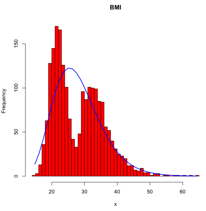
This is clearly unsatisfactory as it does not adequately model the bimodal nature of the data.
Additional research was conducted to find effective ways to initialise the EM algorithm. Many papers suggested clustering approaches such as k-means, but they require well-separated data.
We elected to use a random initialisation strategy to improve the fit, roughly following the ‘alternative method’ from McLachlan et al. (2000, p. 55) or the ‘subset approach’ algorithm described in Schepers (2015). We chose this method as it is easy to implement and produces higher-quality fits than other methods at the expense of computation time Schepers (2015, p. 142). The algorithm proceeds as follows:
for each random start (e.g. 100 times):
    for each mixture component (e.g. two):
        sample p+1 observations from the dataset
        use the ML equations to estimate distribution parameters for those observations
        use those parameters as initial values for the component
    EM fit using those initial parameters and record the log-likelihood of the solution
choose the fit that achieves the highest log-likelihood
\( p \) is the number of parameters that characterise the distribution (2 for the inverse Gaussian distribution). We always set the mixing weight (\( \alpha \)) components to have equal weighting (i.e. 0.5 for a two-component mixture) as we have no information on the true weighting of the components.
Using this algorithm on the BMI dataset, we achieve the following fit:
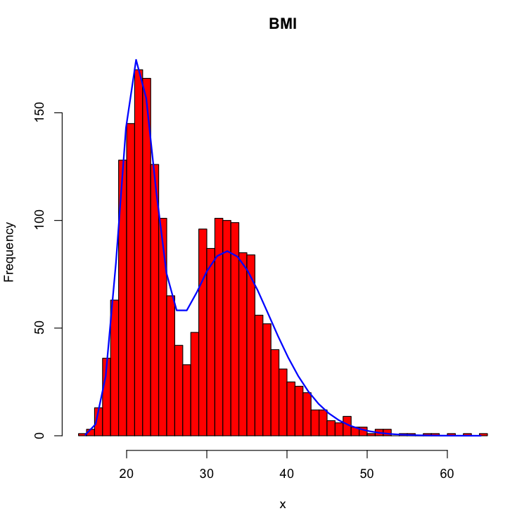
The new model better reflects the bimodal structure of the data.
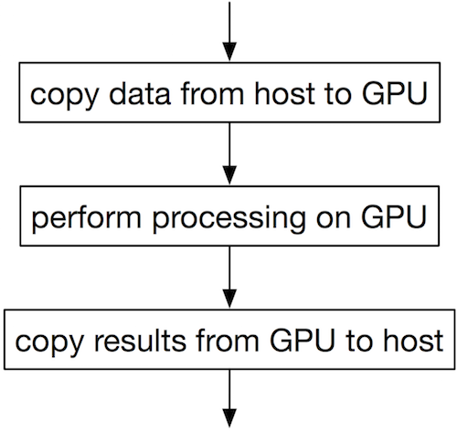
Traditionally, CUDA is used to make a single large task run very quickly. Each observation in the dataset is assigned to a separate CUDA thread; this is termed data parallelism (Wikipedia, 2014). Larger CUDA hardware can process more observations simultaneously. Woolley (2013) states that “To get good performance … You want to have 14K or more threads running concurrently.” To maximise performance, we must make each step run as quickly as possible, even if it is wasteful of machine resources. Most tasks proceed as follows:
bulkem is intended to work efficiently on relatively small datasets with less than 14,000 observations. It expects to see a large number of datasets (thousands) and/or random starts. This suggests that we will need to have multiple tasks running simultaneously on the GPU in order to achieve good performance; task parallelism (Wikipedia, 2015c) is more appropriate. This is a relatively uncommon usage of CUDA hardware; Tzeng et al. (2012) has a brief overview.
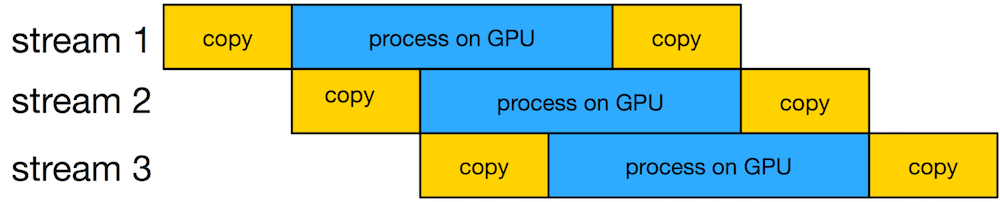
Recent CUDA hardware supports a feature called “streams” (Rennich, 2011) which allows the GPU to perform a number of tasks simultaneously. Recent hardware can simultaneously execute up to 16 CUDA kernels while copying data back and forth between host RAM. We can use streams to:
Assuming sufficient GPU resources are available, the execution flow might look like:
The high-level strategy for bulkem’s CUDA path is therefore:
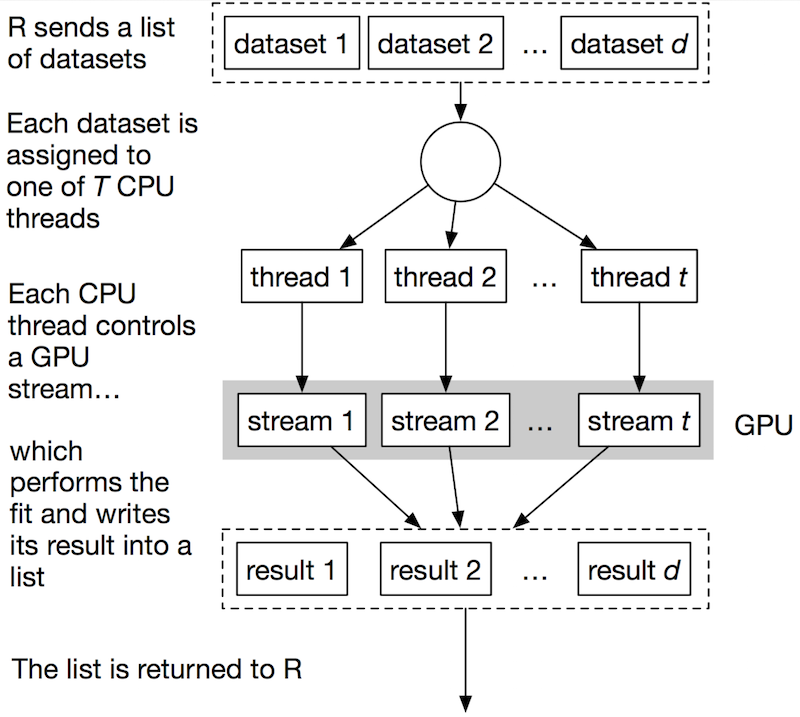
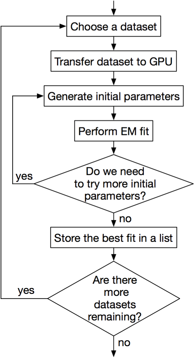
Each CPU thread controls a single CUDA stream. It chooses a dataset to fit, generates many sets of initial parameters and fits each using EM. The bulk of the work of EM fitting is performed on the GPU. After fitting, the best fit is selected and stored.
The final kernel design is guided by the need to minimise the number of kernel launches. The reasons for this are explored in failed kernel designs.
Recall the equations that we need to evaluate to perform a single iteration of the EM algorithm:
$$ \alpha_{\ell}^{new} = \frac{1}{N}\sum_{i=1}^{N}p(\ell|x_{i},\Theta^{g}) $$
$$ \mu_{\ell}^{new} = \frac{\sum_{i=1}^{N}x_{i}p(\ell|x_{i},\Theta^{g})}{\sum_{i=1}^{N}p(\ell|x_{i},\Theta^{g})} $$
$$ \lambda_{\ell}^{new} = \frac{\sum_{i=1}^{N}p(\ell|x_{i},\Theta^{g})}{\sum_{i=1}^{N}\frac{(x_{i}-\mu_{\ell}^{old})^{2}p(\ell|x_{i},\Theta^{g})}{(\mu_{\ell}^{old})^{2}x_{i}}} $$
Each operation within the equations can be classified as either:
Each iteration of the EM algorithm requires \( 2+M \) kernel launches (where \( M \) is the number of mixture components being fit). The first performs the per-observation calculations. At the end of this launch, the operands to every summation are available. This stage is referred to as member_prob_kernel in the source code.
The second launch performs the summation required to evaluate the current log-likelihood. This is called lp_sum_kernel and is described in more detail in fused single launch sum kernel. After this launch, we stop if convergence has been achieved.
The remaining launches perform the summations required to evaluate the new mixture parameter values, again using lp_sum_kernel.
The process to perform a single iteration of the EM algorithm is therefore:
member_prob_kernellp_sum_kernellp_sum_kernel. The update equations can then be evaluated to generate the next iteration’s initial parameter estimates.It took a number of attempts to design a CUDA kernel that performed well. The following table summarises the failed attempts2.
For reference, the pure R implementation took around 80ms to produce each fit using a single CPU core. Each fit runs on the same problem with the same initial conditions, running 100 iterations of the EM algorithm to produce a result.
| Description | Time to fit | Problems |
|---|---|---|
| Basic CUDA C | 2.3ms | Summations were implemented incorrectly, so results were incorrect |
| Using the Thrust API | 80ms | Slow; roughly the same performance as R on CPU |
| Thrust with Streams | 80-290ms | Multiple threads interacted poorly; often slower than before |
| CUB single-threaded | 21ms | Not fast enough to justify use of GPU |
| CUB multi-threaded | 100ms | cudaFuncGetAttributes call using a large amount of time |
| Modify CUB | 15ms | Not fast enough to justify use of GPU |
| Replace CUB with single-launch sum kernel | 3.5ms | Kernel launch time is now the chief bottleneck |
| Fuse multiple summations | 2.5ms | Kernel launch time is now the chief bottleneck |
Broadly, we learned the following:
Kernel launch time is the time that it takes the CPU to launch a kernel on the GPU. Boyer gives measurements showing that calling a CPU function takes about 3.3ns, but launching an asynchronous CUDA kernel takes between 3.0 and 3.9\(\mu\)s – a thousand times longer. Lee et al. (2010) notes that “For GPUs, we found that global inter-thread synchronization is very costly, because it involves a kernel termination and new kernel call overhead from the host.”
This implies that:
Using CUDA streams or CPU threads does not impact this restriction. If many threads are trying to launch a kernel at once, they enter a queue. Only one CPU-GPU operation (a memory copy or kernel launch) can be started at any time, even though many can be in-progress simultaneously.
With small datasets, the kernels do not take long to execute. Kernel launch time then becomes the main determinant of performance. The only way we can reduce launch time is to minimise the number of kernel launches.
The algorithm requires \( 2+M \) summations per iteration. Using the standard CUB or Thrust libraries, two kernel launches are required per summation, giving a total of nine kernel launches for each iteration on a two-component mixture.
To reduce the number of kernel launches required, a new kernel was developed with two important features: it can perform multiple summations with a single kernel launch.
Most sum kernels use a reduction tree, demonstrated on page 3 of Harris (2010). Rather than having a single thread step through each item and keeping a running total, the many cores of CUDA hardware are used. A large number of threads are launched, proportional to the number of items to be summed4. Each thread sums two adjacent items, a task which can be performed extremely quickly. Then, the adjacent items of those summations are summed, and so on until the last two items are summed. The effect of this is that the summation is performed in roughly \( O(\frac{N}{T}\log(N)) \) time. The traditional ‘running sum’ algorithm operates in \( O(N) \) time; far slower on a GPU where \( T \) is large (hundreds or thousands).
For 2 million items, the kernel might be launched across 1 million threads. No existing GPU hardware has this many hardware execution units available, so the launch is split into blocks. Each block runs on the hardware in turn. The blocks are not resident in the GPU at the same time and cannot synchronise with each other. Therefore, multiple kernel launches are needed to achieve synchronisation (Harris, 2010, p. 4).
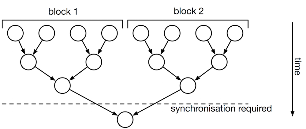
The downside to this algorithm is that each stage must run completely before the next starts, and there is no way to do this except for waiting for the kernel launch to complete. This implies that many kernel launches are required.
The new kernel solves this problem by adding a stage before the reduction tree. If \( T \) threads are launched, the \( t \)th thread calculates
$$ \sum_{i=0}^{\left\lceil N/T\right\rceil }\begin{cases} x_{t+iT} & \text{for t+iT<N}\\ 0 & \text{otherwise} \end{cases} $$
In other words, it sums every \( T \)th element into a \( T \)-wide array. Then, the sum reduction can proceed as per normal. This is slower than the traditional algorithm, but it has the key advantage that global synchronisation is not required. The entire summation can execute with a single kernel launch.
\( T \) can be selected to be any number smaller than the maximum thread block size supported by the CUDA hardware. It is critical that all threads are executed simultaneously (i.e. the kernel must be launched with a grid size of 1).
The M-step of EM requires three summations across \( N \)-sized arrays. These three summations can be performed in a single kernel launch by providing the sum kernel with the details of all three arrays in a single launch, rather than performing three launches. This technique is called Vectored I/O in other contexts (Wikipedia, 2015d).
2 Source code for these can be browsed at https://github.com/ihowson/CUDA-Task-Pipeline
3 Profiling revealed a significant bottleneck in CUB when used in multithreaded applications. This bottleneck has been patched in https://github.com/ihowson/cub/commit/0c90360c9b9c397398a646d689ddd980aa5da811
4 This is a simplified explanation; the curious reader is encouraged to read Harris (2010)
JA Bilmes. A gentle tutorial of the EM algorithm and its application to parameter estimation for Gaussian mixture and hidden Markov models. Technical Report TR-97-021, International Computer Science Institute, 1998.
M Boyer. CUDA kernel overhead. URL http://www.cs.virginia.edu/~mwb7w/cuda_support/kernel_overhead.html.
M Harris. Optimizing parallel reduction in CUDA, Mar 2010. URL http://docs.nvidia.com/cuda/ samples/6_Advanced/reduction/doc/reduction.pdf.
G McLachlan and D Peel. Finite mixture models. John Wiley & Sons, Inc, 2000.
J Hoberock and N Bell. Thrust - parallel algorithms library, Mar 2015. URL http://thrust.github.io/.
MO Prates, CRB Cabral, and VH Lachos. mixsmsn: Fitting finite mixture of scale mixture of skew-normal distributions. Journal of Statistical Software, 54(12), August 2013.
NVIDIA Corporation. CUB, Apr 2015. URL http://nvlabs.github.io/cub/.
S Rennich. CUDA C/C++ streams and concurrency, 2011. URL http://on-demand.gputechconf.com/gtc-express/2011/presentations/StreamsAndConcurrencyWebinar.pdf.
J Schepers. Improved random-starting method for the EM algorithm for finite mixtures of regressions. Behavior Research Methods, 47(1):134–146, Mar 2015.
S Tzeng, A Patney, and JD Owens. GPU task-parallelism: primitives and applications, 2012. URL http://on-demand.gputechconf.com/gtc/2012/presentations/S0138-GPU-Task-Parallelism-Primitives-and-Apps.pdf.
Wikipedia. Data parallelism, Dec 2014. URL http://en.wikipedia.org/wiki/Data_parallelism.
Wikipedia. Inverse gaussian distribution, February 2015a. URL http://en.wikipedia.org/wiki/Inverse_Gaussian_distribution.
Wikipedia. Task parallelism, Mar 2015c. URL http://en.wikipedia.org/wiki/Task_parallelism.
Wikipedia. Vectored I/O, February 2015d. URL http://en.wikipedia.org/wiki/Vectored_I/O.
C Woolley. GPU optimization fundamentals, 2013. URL https://www.olcf.ornl.gov/wp-content/uploads/2013/02/GPU_Opt_Fund-CW1.pdf.